Mon, 16 Dec 2024

Cosmological constant due to quantum corrections to the effective potential

V. A. Filippov ^1,2, R. M. Iakhibbaev ¹, D. I. Kazakov ¹ and D. M. Tolkachev ^*1,3

¹ Bogoliubov Laboratory of Theoretical Physics, Joint Institute for Nuclear Research, Dubna, Russia
² Sarov Branch of Moscow State University, Sarov, Russia
³ B. I. Stepanov Institute of Physics, National Academy of Sciences of Belarus, Minsk, Belarus

DOI: 10.54546/NaturalSciRev.100103

Abstract

Using the generalised renormalisation group formalism, we calculate quantum corrections to the effective potential in \(\alpha\)-attractor models describing the inflationary stage of the Universe evolution. We demonstrate that quantum corrections lead to a change in the initial classical potential, changing its value at the minimum, which can be interpreted as a manifestation of the cosmological constant or dark energy.

Keywords: quantum field theory, inflationary cosmology, the renormalisation group

1. Introduction

Inflationary theory is one of the most promising models for describing the accelerated ex- pansion and properties of the early Universe [1–3]. It solves a number of cosmological problems and is in agreement with modern observational data [4,5]. In the simplest realisation of the inflationary scenario, it is usually assumed that after the Universe leaves the inflationary stage and post-inflationary reheating, it remains in a state with a minimum potential with a value of \(\Lambda \sim 10^{-120} M_{\text{Pl}}^4\), where \(M_{Pl}\) is the Planck mass [6].

In this paper, we demonstrate that taking into account quantum corrections to the effective potential in some cosmological models can lead to a significant change in the classical potential [7,8] and the appearance of a non-zero value of the ground state energy of the Universe, which can be interpreted as a cosmological constant.

In our analysis we use the standard formalism of the effective potential and apply it to the inflationary model of \(\alpha\)-attractors, the so-called \(T\) model [9-11] with the potential

\begin{equation} V(\varphi) = g \tanh^n\left( \frac{\varphi}{\sqrt{6\alpha} M_{\text{Pl}}} \right) = g V_T \label{O} \tag{1}\end{equation}

(we will mainly consider the cases with \(n = 2, 4\), and call them the \(T^2\) and \(T^4\) models, respectively) [12]. Here \(\varphi\) is the inflaton scalar field, \(g = m_{inf}^2 M_{Pl}^2\) is the scale of inflation, where \(m_{inf} \approx 10^{-5}M_{Pl}\) is the mass of the inflaton, and α is a positive number. These models have been successfully used to study the early accelerated expansion phase of the Universe, as well as the dark energy-dominated phase [11,13,14]. The predictions from these models are in agreement with the PLANCK and BICEP/Keck [4,5] observations.

First, we recall the main ideas of the derivation of the generalised renormalisation group equation (RG equation) for the effective potentials of non-renormalisable interactions, which allows us to sum the leading contributions to the effective potential in all orders of perturbation theory. This approach generalises the original work [15]. Then, using these equations, we calculate quantum corrections to the effective potential for a number of cosmological \(T\) models and demonstrate how the non-zero cosmological constant arises as a result of accounting for radiative corrections.

2. Effective potential in the general scalar model

The effective potential \(V_{eff}()\varphi\) can be considered as complementing the classical potential with quantum loop corrections. It is defined as the part of the effective action that does not contain any derivatives [16]. The calculation of the effective potential requires summing all vacuum 1PI diagrams with propagators containing an effective mass term that depends on the classical field \(\varphi: m^2(\varphi)=gv_2(\varphi)\), where \(v_2(\varphi) \equiv \frac{d^2 V(\varphi)}{d\varphi^2}\) and to each vertex there corresponds \(v_n(\varphi) \equiv \frac{d^n V(\varphi)}{d\varphi^n}\), where \(n\) is equal to the number of interior lines at each vertex. Then the effective potential is constructed as a perturbative expansion on the coupling constant \(g\):

\begin{equation} V_{\text{eff}}(\varphi, g) = g \sum_{n=0}^{\infty} (-g)^n V_n(\varphi) . \tag{2}\end{equation}

For regularisation of UV divergences we use dimensional regularisation, when the integration is carried out in \(D = 4 - 2\epsilon\) dimensions of spacetime. The divergent parts of \(\sim 1/ \epsilon^n\) are absorbed by the corresponding counter terms that in renormalisable theories repeat the form of the original Lagrangian. In the non-renormalisable case, these counterterms, on the contrary, do not repeat the original Lagrangian and lead to an infinite number of new structures. This means that in the non-renormalisable case there is infinite arbitrariness, which is not reducible to renormalising a finite number of coupling constants. However, the leading logarithms are free from this arbitrariness and in this paper we focus our attention only on such contributions. For this reason, in the following we omit the singular terms and are concerned only with the logarithmic dependence.

To compute the leading logarithms \(\sim \log^n \left( \frac{m^2}{\mu^2} \right) \), we take advantage of the fact that the coefficient of the singular term \(\sim 1/ \epsilon^n\) coincides with the coefficient of the corresponding logarithm \(\sim \log^n \left( g \, v_2(\varphi) \right)\) giving the contribution to the effective potential. This is true for all orders of PT. Then, by computing the leading poles of \(1/ \epsilon^n\) and replacing the pole by the logarithm, we can obtain the leading contribution to the effective potential.

To obtain the leading poles, we can use the \(R\)-operation [17–19] and the Bogoliubov–Parasiuk theorem [20], which states that, after the subtraction of divergent subgraphs in an arbitrary local theory, the remaining singular part is always local in coordinate space or has a polynomial structure in momentum space. This is always true regardless of whether the theory is renormalisable or non-renormalisable and imposes restrictions on the structure of the singular terms and allows us to obtain recurrence relations for the leading divergences in subsequent orders of perturbation theory [8]. In turn, the recurrence relations can be transformed into a differential equation, which is a generalisation of the RG equation to the non-renormalisable case.

Let us introduce a function \(\Sigma(z, \varphi)\) given by the equation

\begin{equation} \Sigma(\varphi, g) = g \sum_{n=0}^{\infty} (-g)^n \Delta V_n(\varphi), \tag{3}\end{equation}

where \(\Delta V_n\) is the coefficient of the leading pole \(\sim 1/ \epsilon^n\) in the expression for the effective potential. Then the generalised WG equation on the function \(\Sigma(z, \varphi)\) has the following form [8]:

\begin{equation} \frac{\partial \Sigma}{\partial z} = -\frac{1}{4} \left( \frac{\partial^2 \Sigma}{\partial \varphi^2} \right)^2 , \Sigma(0, \varphi) = V_0(\varphi) , \label{D} \tag{4}\end{equation}

where \(z = g/ \epsilon\). To obtain the effective potential, it is enough to replace in the obtained solution the argument \(z\) by the corresponding logarithm:

\begin{equation} V_{\text{eff}}(g, \varphi) = g \Sigma(z, \varphi) \Big|_{{z \to \frac{-g}{16\pi^2}} \log \left( gv_2 / \mu^2 \right)} . \tag{5} \end{equation}

The resulting effective potential contains the leading logarithmic contributions from all orders of perturbation theory.

In general, the above equation is a nonlinear partial derivative equation. Unfortunately, except for the renormalisable case with the \(\varphi^4\) potential, we cannot obtain an analytical solution to this equation and must resort to numerical calculation. The full solution, which takes into account all orders of perturbation theory, usually has smoother behaviour than the one-loop approximation and can include both poles and discontinuities and restore the original symmetry of the classical potential [7].

Let us apply the formalism of the generalised RG to the study of properties of effective potentials of \(\alpha\)-attractor models.

3. Cosmological constant due to quantum corrections

Let us briefly recall the description of \(\alpha\)-attractor models. In [21] it was shown that there exists a wide class of so-called \(\alpha\)-attractor models with hyperbolic geometry of the following kind:

\begin{equation} \label{S} S = \int d^4x \sqrt{-g} \left[ \frac{M_{\rm Pl}^2}{2} R(g) + \frac{1}{2} \frac{\partial_\mu \phi \, \partial^\mu \phi}{ \left(1 - \frac{\phi^2}{6 \alpha M_{\rm Pl}^2} \right)^2 } - V(\phi) \right] \tag{6} \end{equation}

where \(\alpha\) is the free parameter, \(\phi\) is the inflaton field, \(R({g})\) is the scalar curvature, \({g}=\det({g}_{\mu\nu})\), \({g}_{\mu\nu}\) is the spacetime metric, and \(V(\phi)\) is the inflaton potential. The models derived from this action are in good agreement with the observed data.

In the action \eqref{S}, it is possible to convert to the canonical form of the kinetic term. For this purpose, we need to solve the equation \(\partial \phi \bigg/ \left(1 - \frac{\phi^2}{6 \alpha M_{\text{Pl}}^2} \right) = \partial \varphi\) whose solution is \(\varphi = \sqrt{6 \alpha} M_{\text{Pl}} \, \tanh \left( \frac{\varphi}{\sqrt{6 \alpha} M_{\text{Pl}}} \right)\). Then the action \eqref{S} can be written in terms of the canonical field \(\varphi\) with a canonical kinetic term in the following form:

\begin{equation} S = \int d^4x \, \sqrt{-g} \left[ \frac{M_{\text{Pl}}^2}{2} R(g) + \frac{1}{2} \partial_\mu \varphi \, \partial^\mu \varphi - V\left( \sqrt{6 \alpha} M_{\text{Pl}} \tanh \left( \frac{\varphi}{\sqrt{6 \alpha} M_{\text{Pl}}} \right) \right) \right]. \tag{7} \end{equation}

Thus, potentials of type \(V_T = \tanh^n \left( \frac{\varphi}{\sqrt{6 \alpha} M_{\text{Pl}}} \right)\) correspond to degree potentials \(\phi^n\) for non-canonical fields \(\phi\). In the theory of \(\alpha\)-attractors, the degree potentials is generalised to an arbitrary function \(F \left( \tanh \left( \frac{\varphi}{\sqrt{6 \alpha} M_{\text{Pl}}} \right) \right)\) of the hyperbolic tangent [9].

In the following, we consider the equation for the effective potential in \(T\) models focusing on the cases \(n = 2, 4\). To investigate the RG equation \eqref{D} in the theory with the potentials \eqref{O}, we rewrite the function \(\Sigma\) in terms of dimensionless variables \(x = z/M^4_{\text{Pl}}\) and \(y_n = \tanh^n \left( \varphi/\sqrt{6 \alpha} M_{\text{Pl}} \right)\). Then we have

\begin{equation} \Sigma \left( z / M_{\text{Pl}}^4, \tanh^n \left( \varphi / \sqrt{6 \alpha M_{\text{Pl}}} \right) \right) \equiv S(x, y_n). \tag{8} \end{equation}

The function \(S(x,y_n)\) for the general \(T\) model satisfies the RG differential equation

\begin{equation} S_x= -\frac{n^2 y^{2-\frac{4}{n}} \left(y^{2/n}-1\right)^2}{144 \alpha ^2} \left(\left(y^{2/n}+n \left(y^{2/n}-1\right)+1\right) S_y+n y \left(y^{2/n}-1\right) S_{yy}\right)^2.\label{12}\tag{9} \end{equation}

(Here and below we omit the \(n\) index of the variable \(y\).)

The boundary conditions for the \(T^2\) and \(T^4\) models coincide and are chosen such that when \(\varphi \to \infty, \quad \tanh \left( \varphi / \sqrt{6 \alpha M_{\text{Pl}}} \right) \to 1\) the potential reaches a plateau with zero derivative, namely,

\begin{equation} S(0, y) = y, \quad S(x, 1) = 1, \quad S_y(x, 1) = 0 . \tag{10} \end{equation}

Substituting the variables in the original equation \eqref{D}, the generalised RG equation for the function \(S(x, y)\) can be written as follows:

for \(n = 2\)

\begin{equation} S_x = - \frac{(y - 1)^2 \left( (3y - 1) S_y + 2(y - 1) y S_{yy} \right)^2}{36 \alpha^2} , \tag{11} \end{equation}

for \(n = 4\)

\begin{equation} S_x= -\frac{y \left(4 y \left(\sqrt{y}-1\right)^2 S_{yy}+\left(5 y-8 \sqrt{y}+3\right) S_y\right)^2}{9\alpha^2} \label{15}. \tag{12} \end{equation}

The RG equations for these cases were first derived in [8].

Now we can solve these partial differential equations and then choose a line on the surface \((x, y)\) corresponding to the effective potential \(x = - \frac{g}{16 \pi^2} \log \left( g v_2 (\varphi) / \mu^2 \right)\). This line has an additional parameter, the scale \(\mu\). In the renormalisable case, the explicit dependence on this scale is compensated by the implicit dependence on \(\mu\) of the coupling constant \(g\). However, in the non-renormalisable case \(\mu\) remains a free parameter. For different values of \(\mu_2\), one can obtain different behaviour of the potential.

Quantum corrections can significantly affect the behaviour of the potential; in particular, they can “uplift” the minimum, which can be interpreted as the presence of the cosmological constant [8].

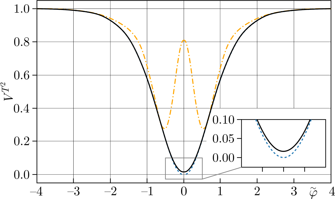
The behaviour of the effective potential for the \(T^2\) model compared to the one-loop case is shown in Fig. 1.

One can see how the one-loop quantum correction leads to a change in the vacuum state of the potential and to the appearance of additional minima (the Coleman–Weinberg mechanism [15]) under the choice of some values of the parameter \(\mu\). However, the sum of all leading quantum corrections smoothes the behaviour of the potential and restores the initial symmetry, as it was in the original paper [15] for the renormalisable theory.

**Figure 1.** Comparison of the classical \(T^2\)-model potential (blue dashed line), the single-loop correction (orange dashed line with a dot), and the effective RG potential (black solid line). For illustrative purposes, when choosing \(g \sim 1, \quad \mu < M_{Pl}, \quad \tilde{\varphi} = \varphi / \sqrt{6} M_{Pl}\).

Figures 2 and 3 show the phase planes for the classical and effective potentials of the \(T^2\) and \(T^4\) models. The blue (grey) region is responsible for the inflation condition. It can be seen that due to quantum corrections the phase trajectories are distorted and new points of attraction (additional minima of the potential) can arise.

It should be noted that, when taking into account quantum corrections, the attractor properties are preserved and the solutions of the inflationary cosmology equations with the obtained effective potentials do not depend globally on the initial conditions. Similar results are obtained in the case \(\mu \gg 1\).

Figure 4 shows a detailed view of the total effective potential for different values of \(\mu\) in the \(T^2\) model. It can be seen that there is an uplift of the potential leading to a non-zero value of the energy at the minimum, which can be interpreted as the appearance of a non-zero value of the cosmological constant \(\Lambda\). As follows from the figure, there are two ways to get a positive value of \(\Lambda\). The first way is when the effective potential has no additional minima but only a rise.

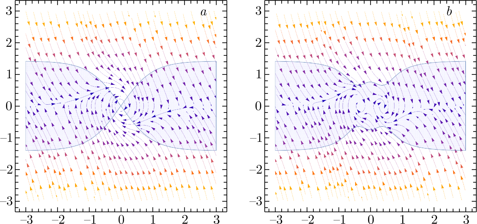
**Figure 2.** Phase portrait for the classical \((a)\) and quantum, in the case of \(\mu \ll 1\!\, (\text{b})\), potential of the \(T^2\) model.

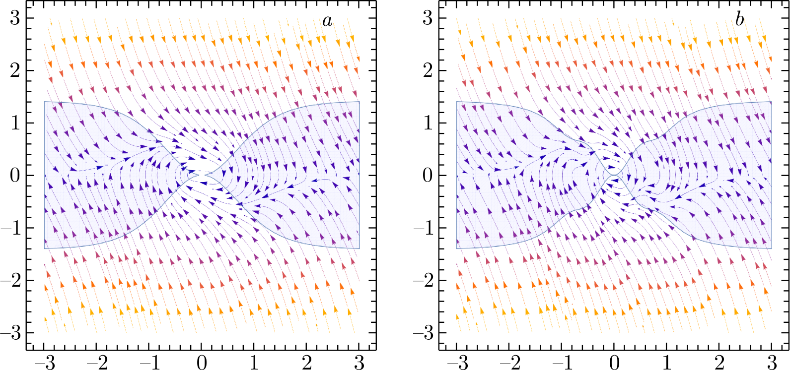
**Figure 3.** Phase portrait for the classical (a) and quantum, in the case of \(\mu \ll 1\!\, (\text{b})\), potential \(T^4\) model.

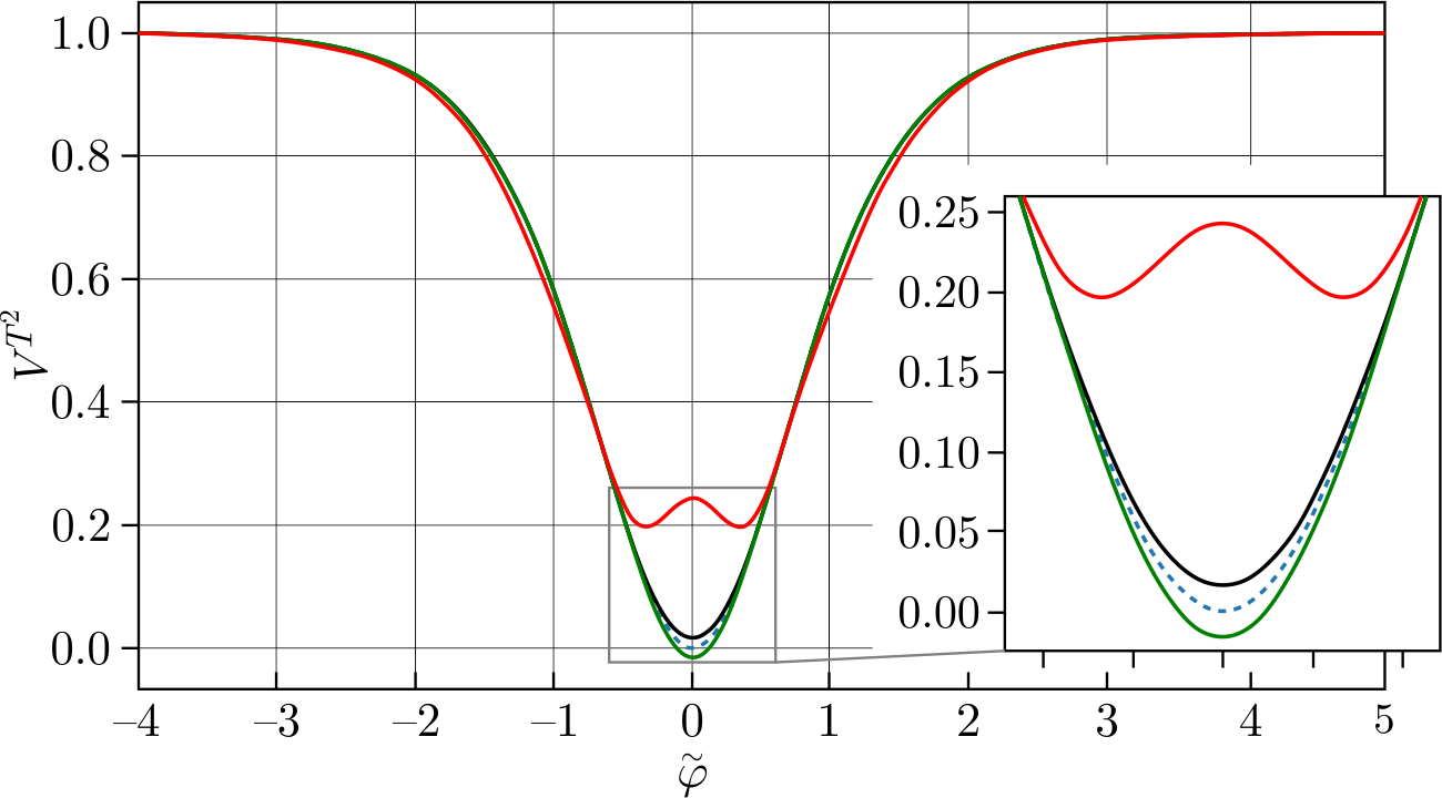
**Figure 4.** \(T^2\)-model potential: variation of \(\mu\). Classical potential (blue dashed line), solid lines denote the all-loop effective potential \(\mu < M_{Pl}\) (black line with dot), \(\mu \ll M_{Pl}\) (red line), and \(\mu > M_{Pl}\) (green line with triangle). The scales are chosen for clarity as follows: \(\tilde{\varphi} = \varphi / \sqrt{6} M_{Pl}\) and \(g = 2, \alpha = 1\)

The second way is when the potential has additional minima in addition to the rise. The choice between these two options depends only on the value of \(\mu\).

If the result does not differ much from the one-loop correction, it is convenient to analyse its properties using the exact formulae for the one-loop potential. The formula for the one-loop effective potential is as follows:

\begin{equation} V_{\text{eff}} = V_0 + \frac{g^2}{16 \pi^2} \frac{v_2^2}{4} \log \left( \frac{g v_2(\varphi)}{\mu^2} \right) , \tag{13} \end{equation}

where\(v_2(\varphi)\) is the second derivative of the classical potential \(V_0\).

As already mentioned, the non-zero value of the potential at the minimum can be interpreted as a cosmological constant given by the relation

\begin{equation} \Lambda=\left.\left[\frac{g^2}{16\pi^2} \frac{v_2^2}{4} \log\left(\frac{g v_2}{\mu^2}\right)\right]\right\vert_{\varphi=\varphi_{\rm vac}} \label{16}. \tag{14} \end{equation}

Applying this condition to the \(T^2\) model, we can obtain an expression for the parameter \(\mu\)

\begin{equation} \mu^2=\frac{g}{3 \alpha M_{\rm Pl}^2}\exp\left(-576 \pi ^2\frac{ \alpha ^2 }{g^2} \Lambda M_{\rm Pl}^4\right). \tag{15} \end{equation}

Choosing the following set of parameters corresponding to the observational data: \(g=10^{-10}M_{\rm Pl}^4\), \(M_{\rm Pl}=(8\pi G)^{-\frac{1}{2}}\), \(\alpha=1\), and \(\Lambda \sim 10^{-120} M_{\rm Pl}^4\), we obtain that \(\mu \approx 10^{-6}M_{\rm Pl}\), which is close enough to the inflaton mass. We can reverse this argument and take a value of \(\mu\) of the order of the inflaton mass and get a sufficiently small value of the cosmological constant.

For potentials of \(T^4\) and higher powers, there is no such uplift as in the case of the \(T^2\) model, as can be seen from the numerical solution shown in Fig. 5. This is due to the fact that \(v_2(0)=0\). Thus, these potentials are not suitable for describing the small cosmological constant.

Returning to the \(T^2\)-model potential, we can calculate the point at which \(\Lambda\) changes sign. This point is found from the condition for changing the sign of the logarithm in \eqref{16} when the argument passes through unity, i.e., \(gv_2/\mu^2_c\vert_{\varphi=\varphi_{\rm vac}}=1\), then the critical point is \(\mu_{c}=\displaystyle\frac{10^{-5}}{\sqrt{3 \alpha}}M_{\rm Pl}\).

When the values of \(\mu<\mu_c\), \(\Lambda\) are positive, when \(\mu>\mu_c\), \(\Lambda\) is negative. This is the scale of the inflaton mass. The critical value of \(\mu\) defines the geometry of spacetime, namely: de Sitter space (dS) when \(\mu>\mu_c\), Minkowski space when \(\mu=\mu_c\), and anti-de Sitter space (AdS) when \(\mu<\mu_c\).

The same takes place if we consider not only the one-loop contribution to the effective potential but also the full solution including all leading logarithms from all loops. In this case, the effective potential has only one minimum at \(\varphi_{\rm vac}=0\). This minimum shows a small uplift for small values of \(\mu\). For very small values of \(\mu\), additional minima can occur, but it is not possible to obtain small values of \(\Lambda\) with such \(\mu\).

In conclusion, at such small values of \(\Lambda\) that follow from the experimental data, the value of \(\mu\) is almost independent of the exact value of \(\Lambda\). Changing \(\Lambda\), consistent with the observed data, affects the value of \(\mu\) only to decimal places. However, if we start increasing \(\Lambda\), we find that starting from about \(\Lambda\approx10^{-23}M_{\rm Pl}^4\), the parameter \(\mu\) depends very strongly on \(\Lambda\) and \(\mu\)

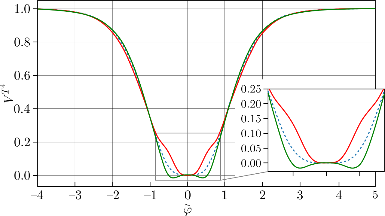
**Figure 5.** Classical potential of the \( T^4 \) model (blue dashed line). Solid lines denote the all-loop effective potential: red at \( \mu^2 \ll M^2_{\text{Pl}} \) and green with a triangle at \( \mu^2 \gg M^2_{\text{Pl}} \). The scales are chosen for clarity as follows: \( \tilde{\varphi} = \varphi / \left(\sqrt{6} M_{\text{Pl}}\right)\) and \( g = 1 \), \( \alpha = 1 \).

rapidly tends to zero at \(\Lambda\approx 10^{-20}M_{\rm Pl}^4\). However, such values of the cosmological constant are unacceptable from the point of view of observational data.

4. Conclusions

In the present study we have investigated the effect of quantum loop corrections on the potentials of \(\alpha\)-attractors used in inflationary cosmology, which from the point of view of quantum field theory are non-renormalisable models. For this purpose, we derive a generalised WG equation whose solution summarises the sequence of leading logarithmic contributions to the effective potential. The full solution depends on the value of the free scaling parameter \(\mu\) and either preserves the potential minimum at the origin or generates new minima. In both cases, the solution can have an uplift of the potential at the minimum. It is important to note that quantum corrections essentially modify the potential only at small values of the field, preserving the attractor properties of the potential.

We interpreted the uplift of the potential as the appearance of the cosmological constant \(\Lambda\) for the model \(T^{2}\). Such an uplift can also be realised for other potentials satisfying the condition \(v_2(0)\neq0\). The obtained value of the free parameter \(\mu\approx10^{-5}M_{\rm Pl}\) calculated in the one-loop approximation lies in the energy region close to the inflaton mass. The numerical estimate obtained from the full equation changes this value only slightly. Since the \(T^4\) potential and higher degree potentials do not satisfy the condition \(v_2(0) \neq 0\), they cannot be used for the mechanism of generation of the cosmological constant \(\Lambda\) described in this paper.

As a result, we can conclude that the cosmological constant \(\Lambda\) can arise as a consequence of quantum loop corrections to the effective potential with some value of the scaling parameter \(\mu\) in the models of cosmological inflation. The value of the cosmological constant \(\Lambda\) can be used to fix the parameter \(\mu\), which can be regarded as a free parameter in non-perturbative theory. It is hoped that the mechanism of radiative corrections can shed light on the existence of dark energy in the early Universe.

Acknowledgements

The authors are grateful to I. Buchbinder, S. Fedoruk, and A. Baushev for valuable discussions.

Conflict of Interest

The authors declare no conflict of interest.