Wed, 12 Feb 2025

Efficient pipeline for plant disease classification

Joint Institute for Nuclear Research, Dubna, Russia

Abstract

Accurate identification of disease and correct treatment policy can save and increase yield. Different deep learning methods have emerged as an effective solution to this problem. Still, the challenges posed by limited datasets and the similarities in disease symptoms make traditional methods, such as transfer learning from models pre-trained on large-scale datasets like ImageNet, less effective. In this study, a self-collected dataset from the DoctorP project, consisting of 46 distinct classes and 2615 images, was utilized. DoctorP is a multifunctional platform for plant disease detection oriented on agricultural and ornamental crop. The platform has different interfaces like mobile applications for iOS and Android, a Telegram bot, and an API for external services. Users and services send photos of the diseased plants in to the platform and can get prediction and treatment recommendation for their case. The platform supports a wide range of disease classification models. MobileNet_v2 and a Triplet loss function were previously used to create models. Extensive increase in the number of disease classes forces new experiment with architectures and training approaches. In the current research, an effective solution based on ConvNeXt architecture and Large Margin Cosine Loss is proposed to classify 46 different plant diseases. The training is executed in limited training dataset conditions. The number of images per class ranges from a minimum of 30 to a maximum of 130. The accuracy and F1-score of the suggested architecture equal to 88.35% and 0.9 that is much better than pure transfer learning or old approach based on Triplet loss. New improved pipeline has been successfully implemented in the DoctorP platform, enhancing its ability to diagnose plant diseases with greater accuracy and reliability.

Keywords: plant disease classification, deep learning, similarity learning, Large Margin Cosine Loss, Triplet loss, ConvNeXt, MobileNet

1. Introduction

Plant disease identification is a critical task for farmers, smallholders, and home gardeners alike. The vast number of diseases and the similarity of their symptoms make it difficult for users to identify the problem and choose the appropriate treatment policy. Deep learning has emerged as an effective solution to this problem. Numerous papers are published annually, exploring various applications of neural networks for disease identification [1–3]. While some researchers propose custom architectures [4,5], transfer learning remains a more popular research area [6–8]. Achieving good results with transfer learning requires extensive domain-specific training data.

There are two types of plant disease datasets. The first type is collected under controlled conditions, where images have a static background, consistent lighting, orientation, and clear separation of subjects. While these datasets, such as PlantVillage [9], are valuable for initial model training, their real-world applicability is limited due to the lack of variability in the conditions under which the images are captured. The second type of dataset is collected in real-world conditions, where images are taken with varying backgrounds, lighting, orientations, and levels of noise. These datasets better reflect the challenges faced in practical applications, making them more suitable for developing models that can generalize well in diverse environments. Although specific crop datasets from real-world conditions can be found on platforms like Kaggle, comprehensive datasets with numerous classes are rare, and the number of images is often limited. In such cases, few-shot learning approaches are increasingly popular. Some of these approaches involve extending datasets using Generative Adversarial Networks (GANs) [10,11], while others use similarity learning. This approach involves determining similarities or differences in data and fine-tuning base networks to better distinguish classes.

In transfer learning, the weights of the base network are typically frozen, and image embeddings are often generated using ImageNet [12] weights. In contrast, similarity learning modifies the base network's weights to better arrange image embeddings in feature space, so that embeddings of the same classes are closer to each other and farther from other classes. Siamese networks [13] are a common solution in plant disease classification. For example, Argüeso et al. [14] demonstrate the benefits of few-shot learning methods over classical fine-tuning transfer learning, using the PlantVillage dataset and Siamese networks with Contrastive [15] and Triplet loss [16] functions. Egusquiza et al. [17] effectively classify 17 disease classes using a real-world dataset, a Siamese network, and a Triplet loss function. In our previous research [18], we used MobileNet_v2 [19] as a backbone and trained it with Triplet loss to classify 25 diseases with over 97% accuracy. However, as the dataset for the DoctorP project (https://doctorp.org/) expanded, the old approaches no longer yielded sufficient results, necessitating the evaluation of new training methods and base architectures.

Loss functions based on angular space, such as SphereFace [20] and ArcFace [21], have shown their effectiveness in face recognition. While Siamese networks operate in Euclidean space, angular span functions work in angular space. Despite this distinction, their objective remains the same: to minimize intra-class variations and maximize inter-class variations in image embeddings. Angular span functions are much less popular in plant disease detection. In [22], the authors propose an EfficientNet-B5 [23] network incorporating ArcFace loss with an adversarial weight perturbation mechanism to classify citrus diseases.

The use of Large Margin Cosine Loss (CosFace) [24], which has shown great results in face recognition, along with ConvNeXt [25] as the base architecture to classify 46 classes of plant diseases, is evaluated in this research.

Appropriate image preprocessing can positively impact model training results. The normalization of pixel values is recommended for imaging modalities, so normalization parameters for the DoctorP dataset will be calculated and used during training. The effect of data augmentation (flips, rotation, brightness, and contrast) on model performance will also be evaluated. The aim of this research is to determine an effective pipeline for plant disease detection using a real-world dataset.

2. Materials and methods

2.1. Dataset

The DoctorP platform, which evolved from the Plant Disease Detection Platform (PDDP) project [26], processes user requests made under various conditions, including different devices, lighting, orientations, and close-ups. These requests have been the primary source of images for dataset updates over the last couple of years. DoctorP handles several models designed for specific tasks. At the first stage of processing user requests, a general model is employed, while specific models for particular crops are used at later stages. This research is based on the dataset for the general model, which includes 46 classes without specifying the crop. These classes are: Alternaria leaf blight, Anthocyanosis, Anthracnose, Ants, Aphid, Black rot, Black spots, Blossom end rot, Canker, Caterpillars, Coccomyces of pome fruits, Colorado beetle, Corn downy mildew, Cyclamen mite, Downy mildew, Dry rot, Edema, Esca, Eyespot, Frost cracks, Grey mold, Gryllotalpa, Healthy, Late blight, Leaf deformation, Leaf miners, Leaf spot, Leaves scorch, Lichen, Loss of foliage turgor, Marginal leaf necrosis, Mealybug, Monilia, Mosaic virus, Northern leaf blight, Polypore, Powdery mildew, Rust, Scale, Shot hole, Shute, Slugs caterpillars effects, Sooty mold, Thrips, Tubercular necrosis, Wireworm.

The dataset includes 2615 images, with the number of images per class ranging from 30 to 130. All images are in RGB format with a resolution of \(256\times256\) pixels. Examples of these images are presented in Figure 1.

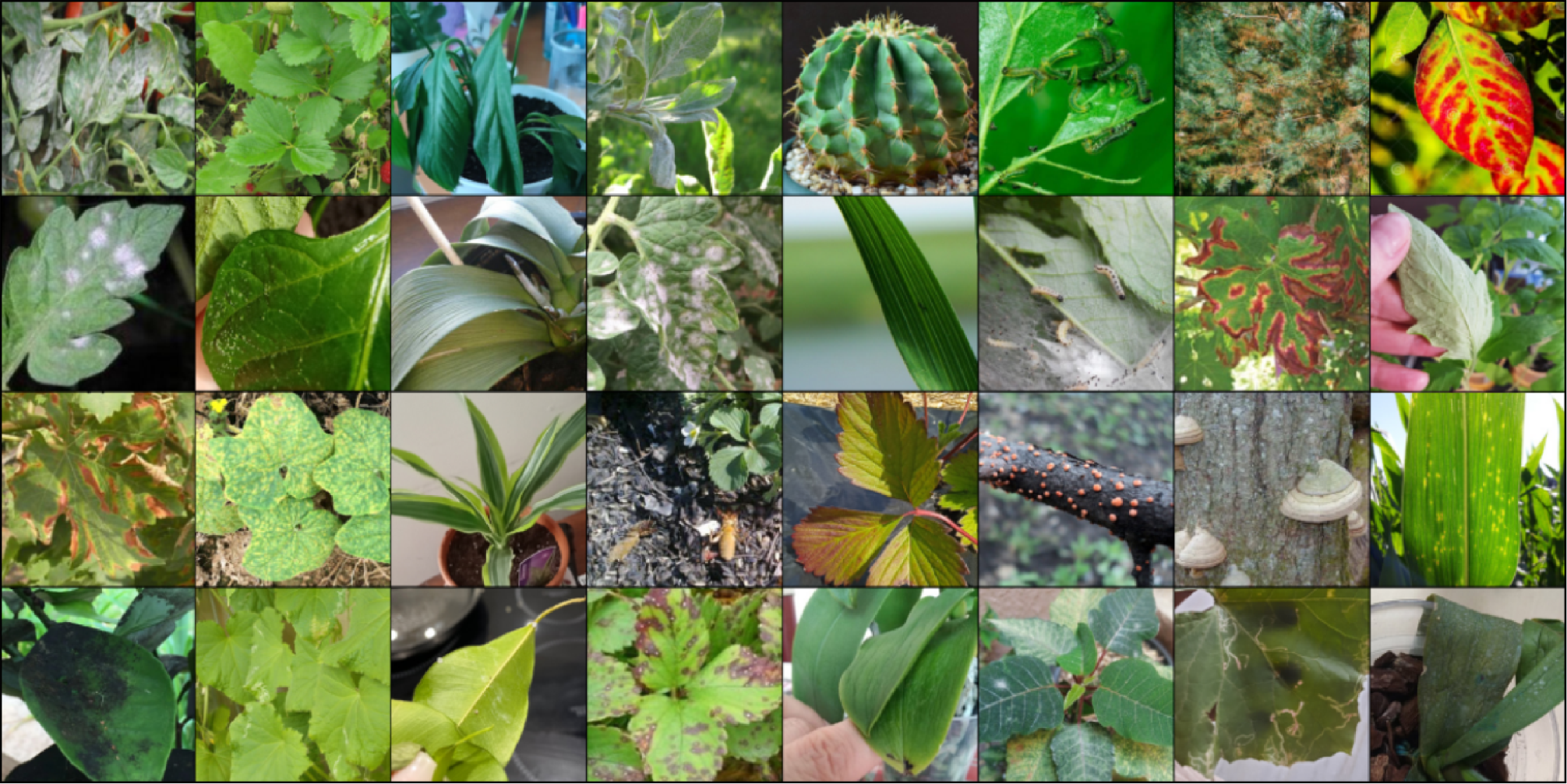
**Figure 1.** Examples of the images in the DoctorP general dataset.

2.2. Methodology

The transfer learning approach involves taking a pre-trained network, freezing its weights, replacing the original classification part with a new one tailored to the new domain, and training it on new data. Since 2012, this has been a popular research area, leading to the introduction of many great architectures. ImageNet, a large dataset used for training and benchmarking new architectures, has been in use since 2010. Most base networks used in transfer learning are pre-trained on ImageNet weights, meaning they are trained on over 14 million images to classify 1000 categories. This extensive training implies a high feature extraction ability of the networks. Previously, MobileNet_v2 was used as the base network in the DoctorP project. It is a lightweight solution presented by Google, achieving 71.9% accuracy (Acc@1) on ImageNet data. Now, ConvNeXt_base, with 84.62% accuracy on ImageNet data, is suggested as the base network. ConvNeXt is significantly larger than MobileNet, but the potential increase in accuracy justifies the higher computational costs. Both architectures, trained using transfer learning, will be compared in this research to evaluate how effectively the base networks, initialized with ImageNet weights, can handle the specific features of plant diseases. To achieve optimal results through transfer learning, the classification part of the new architecture should be trained on hundreds of images per class, which is not always feasible. For instance, in our case, this would require hundreds of photos of different plants with the same disease taken under various conditions. However, in the current situation, we have several classes with as few as 30 images each. In recent years, methods that require less data for training, known as few-shot learning, have become increasingly popular. We used a method involving the determination of similarities or differences in data and fine-tuning base networks to better distinguish classes, known as similarity learning. We used the Triplet loss function to train the feature extractor on our domain data rather than on ImageNet data. The Triplet loss function involves three images during evaluation: an anchor, a positive image from the same class as the anchor, and a negative image from a different class. Triplet loss aims to minimize the distance between the anchor and positive image embeddings while maximizing the distance between the anchor and negative image embeddings. The benefit of training on triplets lies in the number of image combinations that can be compared. The formulation of Triplet loss is typically expressed as in Eq. \eqref{eq1}:

\begin{equation} \label{eq1} L_{\rm triplet}=\max\,(D_{\rm ap} - D_{\rm an}+{\rm margin},0),\tag{1} \end{equation}

here, \(D_{\rm ap}\) is the squared Euclidean distance between the embeddings of the anchor and the positive image, \(D_{\rm an}\) is the squared Euclidean distance between the embeddings of the anchor and the negative image, and margin is a hyperparameter that represents the desired difference between the distance of the anchor-positive pair and the anchor-negative pair. The margin in

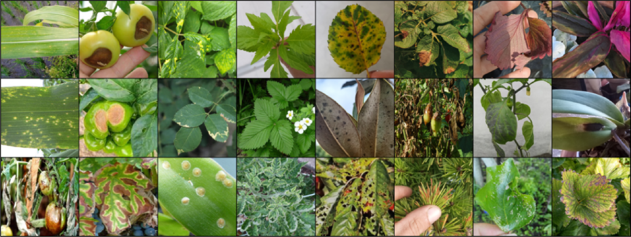
**Figure 2.** Examples of images in the batch for Triplet loss.

the current research is set to 1. To create triplets for training, a random image (anchor) is initially selected. Then, an image from the same class (positive) is chosen (but not the same image), followed by selecting an image from a different class (negative). An example batch of 8 items is presented in Figure2.

Although the Triplet loss function has shown excellent results, there are other methods that offer alternative approaches to Siamese networks. In this research, the CosFace loss function is proposed as a primary alternative to Triplet loss. CosFace reformulates the Softmax loss into a cosine loss by L2 normalizing both features and weight vectors to eliminate radial variations. This normalization allows for the introduction of a cosine margin term, which further maximizes the decision margin in angular space. Consequently, this approach achieves minimal intra-class variance and maximal inter-class variance through normalization and the maximization of the cosine decision margin. This can be formulated as shown in Eq. \eqref{eq2}:

\begin{equation} \label{eq2} L_{\rm cf}=-\frac{1}{N}\sum\limits_{i=1}^N {\log\frac{{\rm e}^{s\left( \cos\left( {\theta }_{y_{i},i} \right)-m \right)}}{{\rm e}^{s\left( \cos\left( {\theta }_{y_{i},i} \right)-m \right)}+\sum\limits_{j{\ne }y_{i}} {\rm e}^{s\cos\left( {\theta }_{j},i \right)} }} ,\tag{2} \end{equation}

subject to

\begin{equation} \begin{aligned} W &= \frac{W^{\ast }}{\left\| W^{\ast } \right\|}, \\ x &= \frac{x^{\ast }}{\left\| x^{\ast } \right\|}, \\ \cos(\theta_{j,i}) &= W_{j}^{T} x_{i}. \end{aligned} \tag{3} \end{equation}

where \(N\) is the number of training samples, \(x_{i}\) is the \(i\)th feature vector corresponding to the ground-truth class of \(y_{i}\), \(W_{j}\) is the weight vector of the \(j\)th class. The \(\theta_{j}\) is the angle between \(W_{j}\) and \(x_{i}\), \(m\) is the margin that controls the cosine margin, and \(s\) is the scale parameter, used to scale the logits for numerical stability and gradient control. In the original paper, the margin \(m\) was varied between 0.25 and 0.45, while the scale \(s\) was set to 64. However, in current research settings, the margin \(m\) is fixed at 0.7 and the scale \(s\) is kept at 64. In this research, we will compare the quality of embeddings extracted by networks trained using CosFace loss and Triplet loss. After training the feature extractors, similar classification layers will be added to the networks, and statistical metrics will be calculated to assess performance. The effects of data augmentation and normalization can vary depending on the data domain and methods used. We will calculate normalization parameters specific to our dataset and apply them during training. Additionally, we will evaluate popular augmentation techniques relevant to our domain, including vertical flip, horizontal flip, and color jitter. The dataset is split into 80% for training and 20% for testing to derive results. Model performance is evaluated using metrics such as accuracy, weighted average precision, recall, and F1-score, with results averaged over 10 runs. Accuracy measures the percentage of correct predictions and is calculated as follows:

\begin{equation} \label{eq4} {\rm Accuracy}=\frac{\rm TP + TN}{\rm TP+FP+TN+FN},\tag{4} \end{equation}

where TP is true positive, FP is false positive, TN is true negative, and FN is false negative. Weighted-average metrics account for the number of samples in each class, calculated as the sum of metrics multiplied by the weights of each class. Basic recall, or True Positive Rate (TPR), is calculated as

\begin{equation} \label{eq5} {\rm Recall}=\frac{\rm TP}{\rm TP+FN}. \tag{5} \end{equation}

Precision is calculated as

\begin{equation} \label{eq6} {\rm Precision}=\frac{\rm TP}{\rm TP+FP}. \end{equation}

The F1-score, which is the harmonic mean of recall and precision, is given by

\begin{equation} \label{eq7} {\rm F}1=\frac{2\times \rm Precision\times Recall}{\rm Precision\times Recall}. \end{equation}

The experiments will be conducted using the heterogeneous infrastructure at the Joint Institute for Nuclear Research [27], utilizing NVIDIA Volta V100 GPUs with 512 GB of RAM.

3. Results and discussion

In the first stage, the weights of the selected backbone networks were frozen. The classification component of the networks was replaced with two linear layers followed by a ReLU activation function. The networks were trained for 50 epochs with a batch size of 64 using the CrossEntropy loss function and the Adam optimizer with a learning rate of 0.0001. No data augmentation was applied, and normalization parameters from ImageNet were used for the training data.

The accuracy and F1-score for MobileNet_v2 were 69.78% and 0.70, respectively, while for ConvNeXt, these metrics were 78.20% and 0.78. It is evident that the larger ConvNeXt outperforms the lighter MobileNet_v2. However, it was uncertain how these networks would perform when fully trained on plant disease images.

In the second stage, the backbone networks were trained with Triplet loss and CosFace loss functions for 30 epochs with a batch size of 64. The size of the embedding vector for each network was set to 1280. The loss chart is presented in Figure 3.

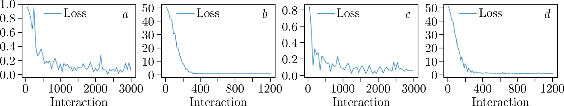
**Figure 3.** Evaluation of loss during 30~epochs of training: \(a\)) MobileNet_v2 with Triplet loss; \(b\)) MobileNet_v2 with CosFace loss; \(c\)) ConvNeXt with Triplet loss; \(it d\)) ConvNeXt with CosFace loss.

Both networks exhibit good convergence and display similar training behavior. The loss curve for the cosine-based loss function is notably smoother, which may be attributed to the specific data preparation process used with Triplet loss. At this stage, accuracy metrics are not available; only loss trends are observed. To gain insights into the nature of the embeddings, visualization techniques such as t-SNE [28] or Principal Component Analysis (PCA) can be employed. t-SNE converts similarities between data points into joint probabilities and aims to minimize the Kullback–Leibler divergence between the joint probabilities of the low-dimensional embedding and the high-dimensional data. 3D plots were utilized to assess the embedding extraction capabilities of the models, as shown in Figure 4.

The dataset comprises 46 classes, which can make color differentiation challenging. Nonetheless, the embeddings are clearly separated regardless of the base network or training approach used.

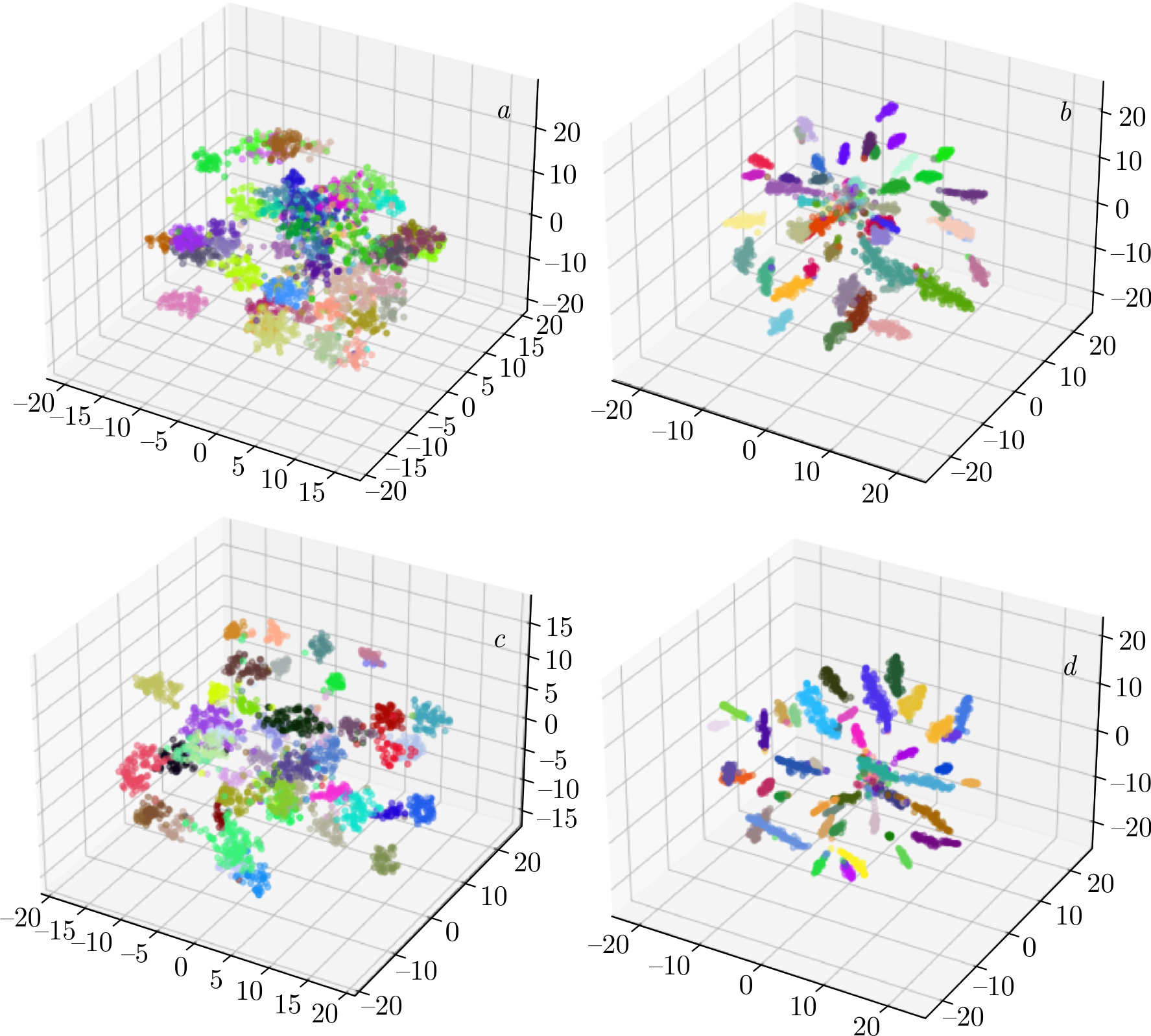
**Figure 4.** t-SNE visualization of embeddings extracted by the models: \(a\)) MobileNet_v2 with Triplet loss; \(b\)) MobileNet_v2 with CosFace loss; \(c\)) ConvNeXt with Triplet loss; \(d\)) ConvNeXt with CosFace loss.

Although this is just one form of visualization, some observations can be made. Embeddings of the same class extracted by the network trained with CosFace loss are positioned closer together no matter which base network was used. At the same time, embeddings extracted using the ConvNeXt architecture show a more distinct distribution in the feature space, with representatives of the same class clustered more closely, while the centers of different classes are more distinctly separated. However, this observation does not guarantee that the networks will exhibit the same performance in classification tasks.

To assess the evaluation metrics, the feature extraction component was integrated with the classification component. This integration involved two linear layers with a ReLU activation function and a dropout rate of 0.2. The networks were trained for 20 epochs using the CrossEntropy loss function and the Adam optimizer with a learning rate of 0.0001. The accuracy and F1-score for MobileNet_v2 were 75.52% and 0.76 for Triplet loss, and 77.43% and 0.78 for CosFace loss. For ConvNeXt_base_v2, the accuracy and F1-score were 82.79% and 0.83 for Triplet loss, and 86.27% and 0.87 for CosFace loss. These results significantly outperform those achieved with simple transfer learning. The more substantial ConvNeXt architecture surpasses MobileNet, leading to further research being focused solely on ConvNeXt.

The next step involved evaluating the effect of data augmentation. Three augmentation techniques were applied: vertical flip and horizontal flip, each with a probability of 0.5, and ColorJitter with parameters set to brightness = (0.5,1.5), contrast = (0.8,1.2), saturation \(=\) 0, and hue \(=\) 0. The experiment revealed a decrease in accuracy to 83.93% and an F1-score of 0.84. Although there are many data augmentation methods and policies available, evaluating the entire list is beyond the scope of this research.

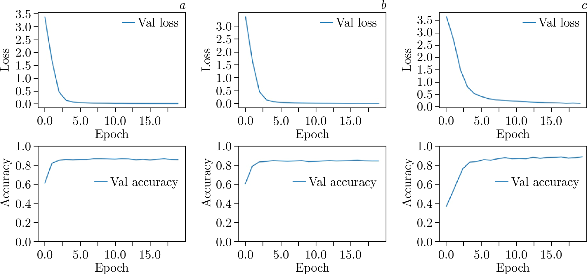
**Figure 5.** Evaluation of model metrics (validation loss and validation accuracy) during the training of ConvNeXt with CosFace loss: \(a\)) without augmentation and normalization; \(b\)) with augmentation but without normalization; \(c\)) without augmentation but with normalization.

**Table 1.** Combined metrics of the models presented in the study (wa — weighted average).
	Accuracy	wa precision	wa recall	wa F1-score
MobileNet_v2 TL	69.78	0.73	0.70	0.70
ConvNeXt_base TL	78.20	0.80	0.78	0.78
MobileNet_v2 Triplet loss	75.52	0.79	0.76	0.76
ConvNeXt_base Triplet loss	82.79	0.85	0.83	0.83
MobileNet_v2 CosFace loss	77.43	0.79	0.77	0.77
ConvNeXt_base CosFace loss	86.27	0.88	0.86	0.86
ConvNeXt_base CosFace loss + augmentation	84.51	0.87	0.85	0.85
ConvNeXt_base CosFace loss + normalization	88.35	0.91	0.90	0.90

Following this, the impact of data normalization was assessed. Normalization parameters for the entire dataset were calculated as follows: \(\text{mean} = [0.4467, 0.4889, 0.3267]\) and \(\text{std} = [0.2299, 0.2224, 0.2289]\). Training the models with these normalization parameters showed a significant improvement, with accuracy increasing to 88.35% and F1-score rising to 0.9. The evaluation of model parameters during training is presented in Figure 5, while the combined metrics for the networks are summarized in Table 1.

It is evident that the metrics are approaching a plateau, leaving little room for further model improvement during training.

Taking into account that there are 46 classes with some having as few as 30 images, an accuracy of 88.35% is a notable result. At this stage of the research, the optimal pipeline for plant disease classification is identified as using the ConvNeXt_base backbone network trained with the Large Margin Cosine Loss on normalized images.

Resource consumption is also a critical consideration. ConvNeXt_base, being larger than MobileNet_v2, requires more training time. Additionally, training with Triplet loss involves processing image triplets, which makes it more time-consuming compared to CosFace loss. Specifically, training MobileNet_v2 with Triplet loss takes approximately 9 min, while training ConvNeXt_base with CosFace loss takes about 33 min. Given that the DoctorP platform involves annual model retraining, 33 min for ConvNeXt_base is acceptable in exchange for superior accuracy.

Future experiments could explore several avenues for further improvement. Incorporating attention mechanisms might enhance model performance by focusing on relevant features. Additionally, Generative Adversarial Networks could be employed to generate synthetic data, which could be useful for expanding the training dataset and potentially improving model performance.

4. Conclusion

Disease classification is a crucial area of research due to its significant impact on food security. The challenges posed by limited datasets and the similarities in disease symptoms make traditional methods like transfer learning less effective. In this study, we utilized a self-collected dataset from the DoctorP project, which includes 46 classes and 2615 images, to identify the most effective pipeline for disease classification. The previously used method, based on MobileNet_v2 and Triplet loss, proved inadequate as the dataset expanded. Our new approach, employing the ConvNeXt_base model trained with CosFace loss on normalized images, achieved an accuracy of 88.35% and an F1-score of 0.9. This improved pipeline has been implemented in the DoctorP platform, enhancing its ability to diagnose issues with agricultural and ornamental crops.

Conflict of Interest

The author declares no conflict of interest.

R. Ramanjot, U. Mittal, A. Wadhawan, J. Singla, N. Z. Jhanjhi, R. M. Ghoniem, S. K. Ray, A. Abdelmaboud, Plant disease detection and classification: A systematic literature review, Sensors 23(2023) 4769. https://doi.org/10.3390/s23104769

S. Muhammad, S. Babar, E. Shaker, A. Akhtar, U. Asad, A. Fayadh, G. Tsanko, H. Tariq, A. Farman, An advanced deep learning models-based plant disease detection: A review of recent research Frontiers in Plant Science 14 (2023). https://doi.org/10.3389/fpls.2023.1158933

J. V. A. Porto, A. C. Dorsa, V. A. M. Weber, K. R. A. Porto, H. Pistori, Usage of few-shot learning and meta-learning in agriculture: A literature review, Smart Agricultural Technology 5 (2023) 100307. https://doi.org/10.1016/j.atech.2023.100307

M. Dyrmann, H. Karstoft, H. S. Midtiby, Plant species classification using deep convolutional neural networks, Biosystems Engineering 151 (2016) 72–80. https://doi.org/10.1016/j.biosystemseng.2016.08.002

A. K. Abasi, S. N. Makhadmeh, O. A. Alomari, M. Tubishat, H. J. Mohammed, Enhancing rice leaf disease classification: A customized convolutional neural network approach, Sustainability 15 (2023) 15039. https://doi.org/10.3390/su152015039

K. P. Ferentinos, Deep learning models for plant disease detection and diagnosis, Computers and Electronics in Agriculture 145 (2018) 311–318.https://doi.org/10.1016/j.compag.2018.01.009

A. Picon, M. Seitz, A. Alvarez-Gila, P. Mohnke, A. Ortiz-Barredo, J. Echazarra, Crop conditional convolutional neural networks for massive multi-crop plant disease classification over cell phone acquired images taken on real field conditions, Computers and Electronics in Agriculture 167 (2019) 105093.https://doi.org/10.1016/j.compag.2019.105093

F. Adnan, M. J. Awan, A. Mahmoud, H. Nobanee, A. Yasin, A. M. Zain, EfficientNetB3-adaptive augmented deep learning (AADL) for multi-class plant disease classification, IEEE Access 11 (2023) 85426–85440.https://doi.org/10.1109/ACCESS.2023.3303131

D. P. Hughes, M. Salathe, An open access repository of images on plant health to enable the development of mobile disease diagnostics, arXiv (2015).https://arxiv.org/abs/1511.08060

Y. Lu, X. Tao, N. Zeng, J. Du, R. Shang, Enhanced CNN classification capability for small rice disease datasets using progressive WGAN-GP: Algorithms and applications, Remote Sensing 15 (2023) 1789.https://doi.org/10.3390/rs15071789

Y. Wang, Y. Yin, Y. Li, T. Qu, Z. Guo, M. Peng, S. Jia, Q. Wang, W. Zhang, F. Li, Classification of plant leaf disease recognition based on self-supervised learning, Agronomy 14 (2024) 500.https://doi.org/10.3390/agronomy14030500

J. Deng, W. Dong, R. Socher, L. J. Li, K. Li, L. Fei-Fei, ImageNet: A large-scale hierarchical image database, in: Proceedings of the IEEE Conference on Computer Vision and Pattern Recognition, Miami, FL, USA, 2009, pp. 248–255.https://doi.org/10.1109/CVPR.2009.5206848

G. Koch, R. Zemel, R. Salakhutdinov, Siamese neural networks for one-shot image recognition, in: Proceedings of the ICML Deep Learning Workshop, Lille, France, 2015, pp. 1–8.

D. Arg ̈ueso, A. Picon, U. Irusta, A. Medela, M. G. San-Emeterio, A. Bereciartua, A. Alvarez- Gila, Few-shot learning approach for plant disease classification using images taken in the field, Computers and Electronics in Agriculture 175 (2020) 105542.https://doi.org/10.1016/j.compag.2020.105542

S. Chopra, R. Hadsell, Y. LeCun, Learning a similarity metric discriminatively, with application to face verification, in: Proceedings of the IEEE Conference on Computer Vision and Pattern Recognition, San Diego, CA, USA, 2005, pp. 539–546. https://doi.org/10.1109/CVPR.2005.202

F. Schroff, D. Kalenichenko, J. Philbin, FaceNet: A unified embedding for face recognition and clustering, in: Proceedings of the IEEE Conference on Computer Vision and Pattern Recognition, Boston, MA, USA, 2015, pp. 815–823. https://doi.org/10.1109/CVPR.2015.7298682

I. Egusquiza, A. Picon, U. Irusta, A. Bereciartua-Perez, T. Eggers, C. Klukas, E. Aramendi, R. Navarra-Mestre, Analysis of few-shot techniques for fungal plant disease classification and evaluation of clustering capabilities over real datasets, Frontiers in Plant Science 13 (2022) 813237.https://doi.org/10.3389/fpls.2022.813237

A. Uzhinskiy, G. Ososkov, P. Goncharov, A. Nechaevskiy, A. Smetanin, One-shot learning with triplet loss for vegetation classification tasks, Computer Optics 45 (2021) 608–614.

M. Sandler, A. Howard, Z. Zhu, A. Zhmoginov, L.-C. Chen, MobileNetV2: Inverted residuals and linear bottlenecks, arXiv (2018). https://arxiv.org/abs/1801.04381

W. Liu, Y. Wen, Z. Yu, M. Li, S. Raj, L. Song, SphereFace: Deep hypersphere embedding for face recognition, arXiv (2017).https://arxiv.org/abs/1704.08063

J. Deng, J. Guo, J. Yang, N. Xue, I. Kotsia, S. Zafeiriou, ArcFace: Additive angular margin loss for deep face recognition, arXiv (2018).https://arxiv.org/abs/1801.07698

Q. Dai, Y. Guo, Z. Li, S. Song, S. Lyu, D. Sun, Y. Wang, Z. Chen, Citrus disease image generation and classification based on improved FastGAN and EfficientNet-B5, Agronomy 13 (2023) 988.https://doi.org/10.3390/agronomy13040988

M. Tan, Q. V. Le, EfficientNet: Rethinking model scaling for convolutional neural networks, arXiv (2019).https://arxiv.org/abs/1905.11946

H. Wang, Y. Wang, Z. Zhou, X. Ji, D. Gong, J. Zhou, Z. Li, W. Liu, CosFace: Large Margin Cosine Loss for deep face recognition, arXiv (2018).https://arxiv.org/abs/1801.09414

Z. Liu, H. Mao, C.-Y. Wu, C. Feichtenhofer, T. Darrell, S. Xie, A ConvNet for the 2020s, arXiv (2022).https://arxiv.org/abs/2201.03545

G. Ososkov, A. Nechaevskiy, A. Uzhinskiy, P. Goncharov, Architecture and basic principles of the multifunctional platform for plant disease detection, in: CEUR Workshop Proceedings, GRID 2018 — Selected Papers of the 8th International Conference “Distributed Computing and Grid- Technologies in Science and Education”, 2018, pp. 200–206.

M. Zuev, Y. Butenko, M. Cosi ́c, A. Nechaevskiy, D. Podgainy, I. Rahmonov, A. Stadnik, O. Streltsova, ML/DL/HPC ecosystem of the HybriLIT heterogeneous platform (MLIT JINR): New opportunities for applied research, in: Proceedings of the 6th International Workshop on Deep Learning in Computational Physics (DLCP2022), 2022.

L. J. P. Maaten, G. E. Hinton, Visualizing high-dimensional data using t-SNE, Journal of Machine Learning Research 9 (2008) 2579–2605.