Three-loop moments and spectral density of photonpolarization function in QED

¹ Bogoliubov Laboratory of Theoretical Physics, Joint Institute for Nuclear Research, Dubna, Russia
² Budker Institute of Nuclear Physics, Novosibirsk, Russia
³ Skobeltsyn Institute of Nuclear Physics, Moscow State University, Moscow, Russia

Abstract

We calculate three-loop photon spectral density in QED with Ndifferent species of electrons. The obtained results were expressed in terms of iterated integrals, which can be either reduced to Goncharov’s polylogarithms or written in terms of one-fold integrals of harmonic polylogarithms and complete elliptic integrals. In addition, we provide threshold and high-energy asymptotics of the calculated spectral density. It is shown that the use of the obtained spectral density correctly reproduces separately calculated moments of corresponding photon polarization operator.

Keywords: photon polarization operator, radiative corrections, quantum electrodynamics

1. Introduction

Recent advances in the precision of low-energy \(e^+e^−\) experiments (VEPP-2M, DAFNE,BEPC, PEP-II and KEKB colliders) call for a comparable precision of theoretical predictions.In particular, one has to compute complete NNLO corrections to both leptonic (for example,\(μ^+μ^−\)) and hadronic (for example,\(π^+π^−\)) production. In the present paper we take a first step towards calculation of NNLO QED corrections to the \(e^+e^− \to μ^+μ^−\) total production cross section, which is a key process for the center-of-mass energy calibration at present and future \(e^+e^−\) colliders. Specifically, we will be interested in contribution related to photon vacuum polarization. At three loops the photon spectral density contains NNLO contribution to \(e^+e^− \to μ^+μ^−\), NLO contribution to \(e^+e^− \to μ^+μ^− + γ\), and LO contributions to \(e^+e^− \to μ^+μ^− + 2γ\) and \(e^+e^− \to μ^+μ^−μ^+μ^−\) total production cross sections. All these contributions can be separated from each other, but in the present paper we will restrict ourselves only to their sum. Such a restricted setup nevertheless allows us to test different approximate threshold and high-energy expansions of photon spectral density by comparing them with exact results and make conclusions on the applicability of similar expansions for the calculation of full cross sections1. The latter should greatly reduce the complexity of future full calculations. Moreover,the provided techniques can be further used for the calculation of NNLO corrections to the \(e^+e^− \to μ^+μ^−\) production cross section in the framework of scalar QED.

The photon spectral density can be conveniently defined as a discontinuity of photon polarization operator \(Π(s)\). The latter is given by an extra factor \((1 + Π(s))\) in the denominator of renormalized photon propagator and is one of the several fundamental quantities arising ina study of quantum electrodynamics. At present we have exact results for one- and two-loop contributions [1,2]. However, starting from three loops there are only approximate results [3–6]. For example, the derivation of Baikov and Broadhurst [3] employs a simple Pad`e ap-proximation for three-loop contribution using a few terms of the asymptotic expansions near 3 special points: \(s= 0,4m^2,∞\) (\(m\) is the electron mass).

In the present paper we will provide for the first time exact as well as approximate threshold and high-energy results for three-loop photon spectral density. To check the obtained exact and asymptotic expressions for spectral density, the latter are used for the calculation of the moments of photon polarization operator. The comparison is performed with similar moments calculated from generalized Frobenius power series expansion of photon polarization operator at \(s= 0\). Also, the knowledge of exact photon spectral density already allows us to check the importance of the missed threshold \((s= 16m^2)\) in the reconstruction analysis of three-loop photon polarization operator performed by Baikov and Broadhurst.

2. Spectral density calculation

To calculate three-loop QED photon spectral density \(ρ(s)\), we followed standard procedure:

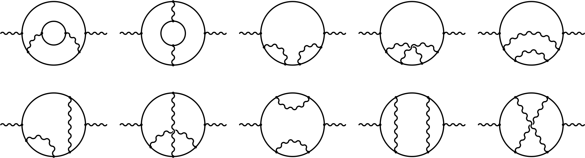
• generation of Feynman diagrams\(^2\) for photon self-energy (see Fig.1)
• application of projector to extract photon polarization operator \(Π(s)\) and subsequent mapping of scalar integrals to the minimal set of prototype integrals;
• IBP reduction [8,9] of prototype integrals to the set of master integrals and application of bipartite cuts with Cutkosky rules for the latter;
• substitution of expressions for cut master integrals\(^3\) [10,11] and renormalization.

This way, considering QED with \(N\) electron flavors\(^4\) and using on-shell renormalization scheme\(^5\),we get

where\(^6\) \( \left( \bar{s} = \frac{s}{m^2}, \quad \beta = \sqrt{1 - \frac{4}{\bar{s}}} \right) \),

The three-loop contribution \(\rho^{(3)}(s)\) can be naturally separated into two pieces corresponding to \(2m\) and \(4m\) cuts, so that we have

where

and

Here, \(f(\bar{s})\) is the function given in Appendix B and defined in terms of products of complete elliptic integrals of first kind. The expressions for \(c_i\) coefficients can be found in Appendix C. The iterated integrals with \(l_i\) weights only can be straightforwardly rewritten in terms of Goncharov’s multiple polylogarithms, while those with elliptic kernels (\(r_i\) or \( r̃_i\) weights) in terms of one-fold integrals of harmonic polylogarithms and complete elliptic integrals as shown in [10]. The latter representations are already well suited for numerical evaluations. However, as we will see in the next section, much more faster numerics in the whole range of \(s\) values can be obtained with threshold and high-energy expansions of spectral densities.

3. Asymptotics and checks

The asymptotic expansions of obtained spectral densities can be done through the asymptotic expansions of iterated integrals as described in [10]. While it is straightforward to do asymptotic expansions in the threshold cases, the high-energy expansions are more involved and may require finding PLSQ relations [12] for polylogarithmic constants at unity argument.To avoid this, one can obtain required asymptotic expansions for master integrals themselves through the Frobenius solution of corresponding differential equations\(^7\). The calculation of spectral densities with the asymptotic expressions for cut master integrals then gives

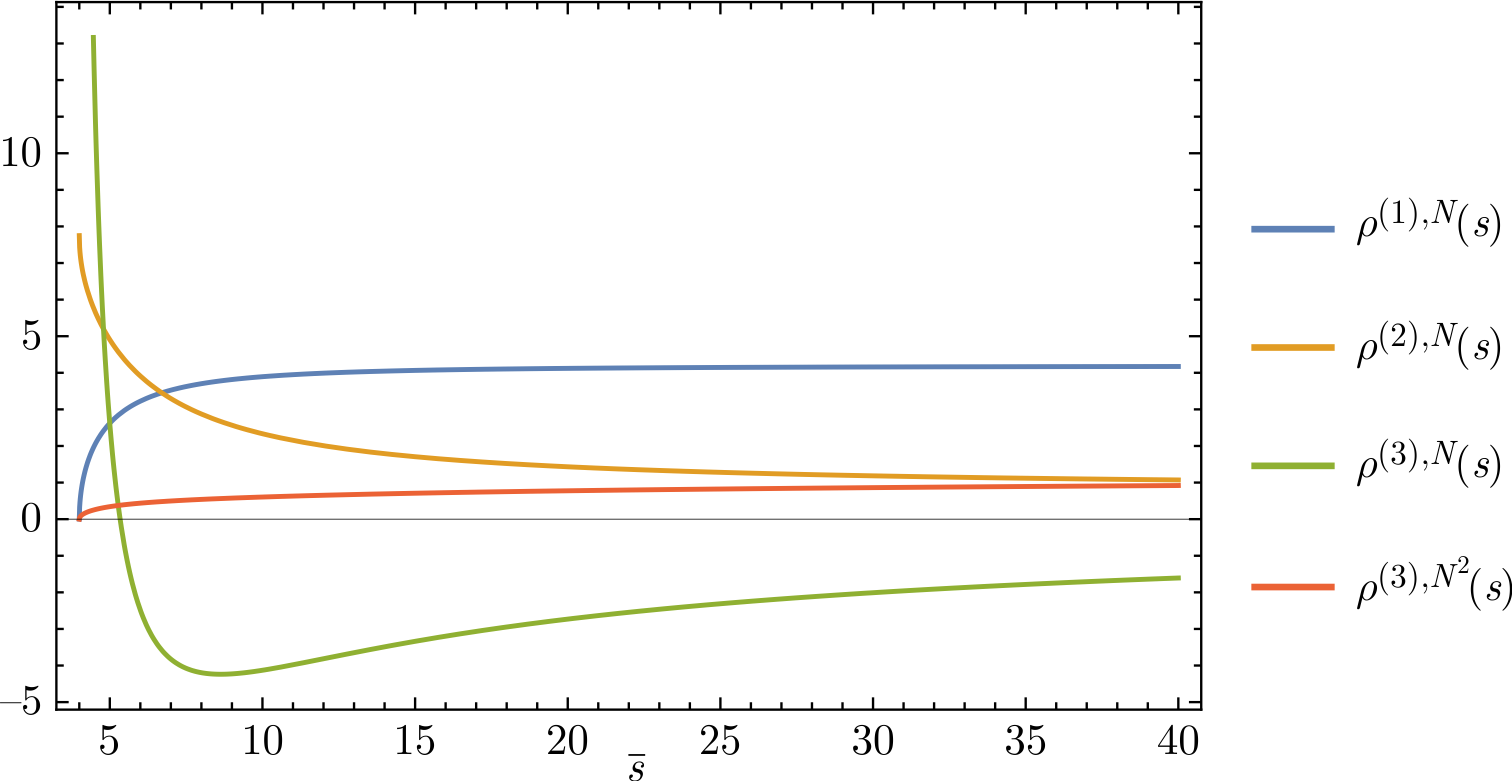
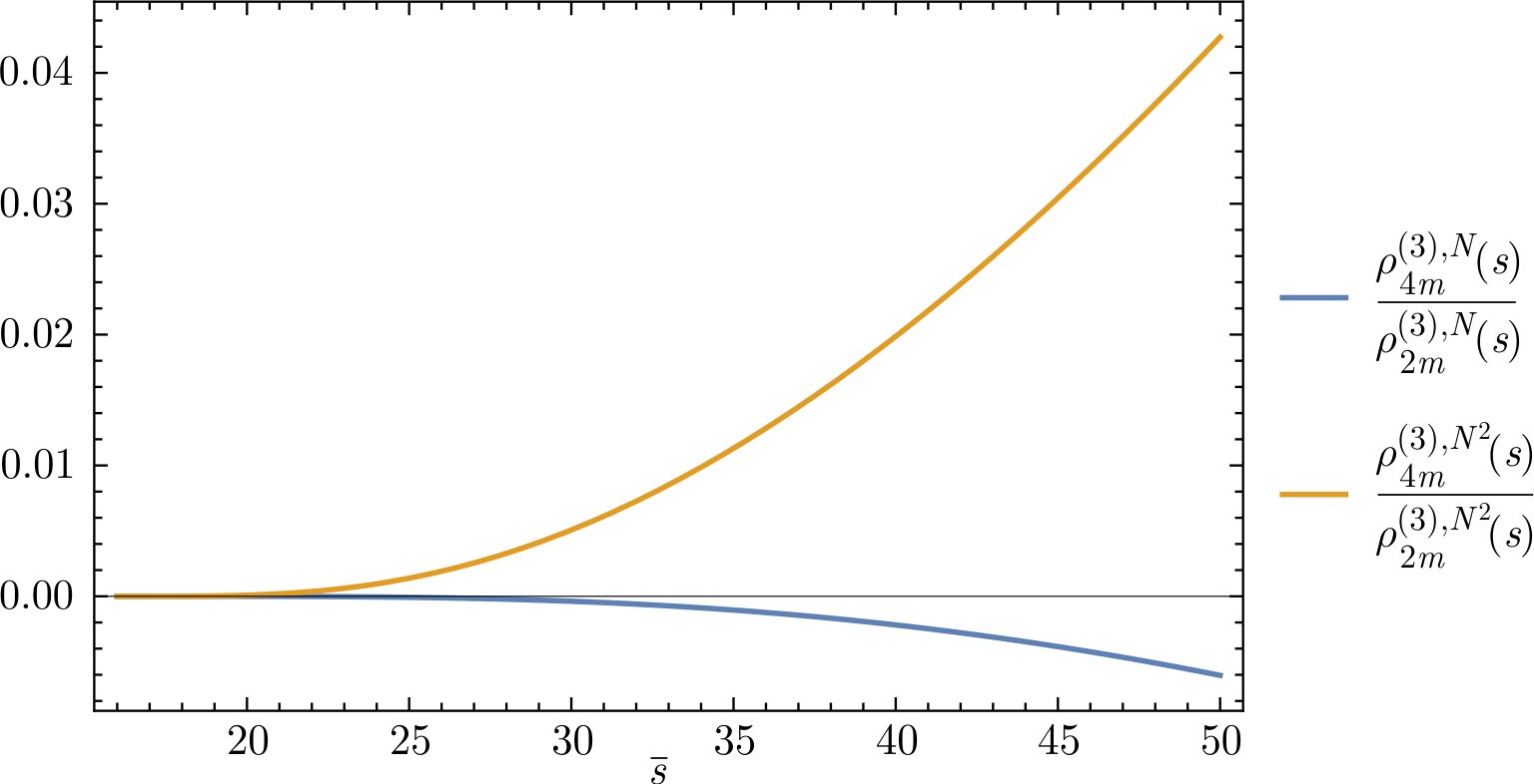
and results with more terms in the expansions can be found in accompanying Mathematica notebook. Using the latter, it is easy to get a very accurate representation of the above spectral densities for the whole range of \(\bar s\) values. The corresponding plot of different contributions can be found in Fig. 2. It is also interesting to compare the ratio of \(4m\) and \(2m\) cuts contributions to three-loop spectral density in the region of \(\bar s\) values where mass effects become important. The corresponding plot can be found in Fig. 3. From the latter we may conclude that the account of second threshold \(\bar s = 16\) missed in the reconstruction of photon polarization operator performed in [3] is not actually important.

To check the obtained results for the spectral densities, we first performed the whole calculation in an arbitrary gauge and made sure that the gauge dependence of spectral densities

cancels. Second, we have numerically checked that the first three moments\(^8\) \(M_n\) of polarization operator computed in [3] agree with a very high precision (at least 15 digits) with moments obtained with the use of our spectral densities and dispersion relation

Moreover, we performed a comparison with additionally calculated 97 moments, see Appendix D and accompanying Mathematica notebook. This latter calculation is similar to the one we did for spectral densities except that in this case we used uncut master integrals. The Frobenius solutions for the latter can be easily obtained from corresponding differential equations using standard techniques. Next, with the computed spectral densities, we can deduce approximate analytical expressions for moments with large n values. Indeed, making variable change in the dispersion relation from \(s'\) to \(\beta' = 1 - \sqrt{{4m^2}/{s'}}\), it is easy to see that

where for large n values the largest contribution to the integral comes from small \(\beta'\) values and for three-loop spectral density it is sufficient to consider only \(2m\) cut contribution. At one loop due to finite \(\beta'\) expansion of spectral density, this expression is actually exact and we have

At two and three loops the formulae are approximate and are given by

where \(d\) coefficients are defined as

Here, order\(_\beta\) is the expansion order in \(\beta\) of corresponding spectral densities, and

is the usual polygamma function. With order\(_\beta\) = 80 the approximate expression for \(M_1^{(2)}\) is accurate with 0.04 percent level, \(M_{10}^{(2)}\) with \(10^{−10}\) percent level and \(M_{50}^{(2)}\) with \(10^{−26}\) percent level. For order\(_\beta\) = 10 the corresponding errors are \(2,10^{(−3)}\) and \(10^{−6}\) percent. With order\(_\beta\) = 120 the accuracy for approximate expression of \(M_1^{(3)}\) is 0.4 percent, for \(M_{10}^{(3)}\) it is \(10^{−10}\) percent, and for \(M_{50}^{(3)}\) it is \(10^{−32}\) percent. For lower value of order\(_\beta\) = 10 the corresponding values are \(13, 10^{−30}\) and \(10^{−7}\) percent. So, we see that for sufficiently large values of moments our approximate formulae are very accurate except for a few first moments.

4. Conclusion

In the present paper we have performed calculation of three-loop photon spectral density in the framework of QED with \(N\) different electron flavors. The obtained results contain both exact and asymptotic expressions. The exact results were written in terms of iterated integrals, which reduce either to Goncharov’s polylogarithms or to one-fold integrals of harmonic polylogarithms and complete elliptic integrals. The asymptotic expressions, on the other hand, allow us to have very accurate expressions for the spectral density in the whole s range. It is shown that the obtained spectral density correctly reproduces first hundred moments of the photon polarization operator. In addition, we supply approximate analytical formulae for the moments of the photon polarization operator. The latter are very accurate for almost all moments except maybe the first few.

Finally, we would like to note that the performed calculation showed that for practical purposes it is sufficient to know required master integrals in terms of their asymptotic threshold and high-energy expansions. The latter can be easily obtained from generalized Frobenius solutions to corresponding differential equations. This gives us a hope that similar approximate solutions will also be applicable to other master integrals required to obtain full NNLO contribution for \(e^+e^− \to μ^+μ^−\) total production cross section.

Acknowledgments

The author is grateful to R. N. Lee for interest in this work and valuable discussions. This work was supported by the Russian Science Foundation, grant 20-12-00205.

Conflict of Interest

The author declares no conflict of interest.

Appendix A. On-shell renormalization constants

The required on-shell renormalization constants for QED with N similar electron species can be extracted from renormalization of two-loop photon and electron self-energies. For photon wave function renormalization \(A_0=Z_AA\) we have \( \left( \alpha = \frac{e^2}{4\pi} \right) \)

where

Here \(m\) is the electron pole mass, \(\mu\) is the dimensional parameter entering dimensional regularization, and \(e\) is the on-shell electron charge at \(q^2 = 0\). The charge renormalization constant \( \left( \alpha_0 = Z_\alpha \alpha \mu^{2\varepsilon} \right) \) is then obtained using Ward identity as

Similarly, from electron self-energy for on-shell mass renormalization constant \( \left( m_0 = Z_m m \right) \) we get

where

and \(a_4 = \text{Li}_4\left(\frac{1}{2}\right) = \sum_{n=1}^{\infty} \frac{1}{2^n n^4}\). Note that at \(N = 1\) these renormalization constants reduce to already known QED values [13–15].

Appendix B. Notation for iterated integrals

The iterated integrals present in the current paper involve the following set of integration kernels or weights:

where

and \(K\) is complete elliptic integral of first kind. The required iterated integrals are then defined as

where weights \(w_k(s)\) take values from the set above.

Appendix C. Expressions for \(c_i\) coefficients

For \(c_i\) coefficients present in the expression for three-loop photon spectral density, we have the following expressions:

Appendix D. Moments of photon correlation function

The moments of photon correlation function are given by

where

and the first five moments at one, two and three loops are given by

The additional moments up to \(n\) = 100 can be found in accompanying Mathematica notebook.